 .
.GRAF (Genetic Relationship And Fingerprinting) is a package useful for analyzing and visualizing genotype data from genome-wide association studies. The latest version, GRAF 2.4, includes three main features:
    1. subject relationship inference (GRAF-rel);
    2. subject ancestry (or population structure) inference (GRAF-pop);
    3. subject sex determination using genotypes (GRAF-sex).
graf to calculate the relationships, predict subject ancestry and determine sexes, and four auxiliary Perl programs: PlotGraf.pl, PlotPopulations.pl and PlotSexCheckResults.pl to visualize the results, and SetRsIdsInBimFile.pl to convert SNP IDs in .bim file into RS IDs so that it can be taken by graf. Note that PlotGraf.pl, PlotPopulations.pl and PlotSexCheckResults.pl require that GD Graphics Library (http://search.cpan.org/~lds/GD-1.38/GD.pm) be installed.
The above executables and other files are included in the GRAF package GrafPkg.tar.gz and visible as separate files after the user executes the command:
tar zxvf GrafPkg.tar.gz
GRAF-rel analyzes the genotypes of all the 10,000 fingerprinting SNPs (distributed as the file FP_SNPs.txt) and calculates the all genotype mismatch rate (AGMR) and the homozygous genotype mismatch rate (HGMR) for each pair of samples (Jin et al., 2017). AGMR is the percentage of SNPs on which the two genotypes are not identical, while HGMR is the genotype mismatch rate when only the SNPs with homozygous calls for both samples are considered.
graf compares the genotypes of all pairs of subjects and finds and reports the closely related pairs, while PlotGraf.pl takes the file generated by graf and plots graphs to show the distributions of HGMR and AGMR values.
In most usages, graf expects as input one or more genotype datasets in PLINK format, i.e., .bed, .bim, and .fam files that share a prefix in their names. However, since multiple samples can be collected from one subject and the subject sample mapping information is not stored in datasets in PLINK, graf reads subject sample mapping information from an SSM file and pedigree information from a pedigree file . The IDs (second column, no column header) in the PLINK .fam file are read as sample IDs by graf. If subject IDs are the same as sample IDs, then no SSM file is necessary, and graf will read the pedigree information from the PLINK .fam file.
However, if any of the sample IDs are different from their corresponding subject IDs, then an SSM file should be passed to graf. The SSM file should be a tab-delimited plain text file with a sample column and a subject column (with column headers—see dbGaP submission guide). When an SSM file is provided, a pedigree file (see dbGaP submission guide) should also be provided to pass the pedigree information to graf. The pedigree file should be a tab-delimited plain text file with at least the following 5 columns (with a column header row):
    1. FAMILY_ID
    2. SUBJECT_ID
    3. FATHER
    4. MOTHER
    5. SEX (1 = male; 2 = female; 0 or NULL = unknown)

    'SUBJECT_ID', 'FATHER', and 'MOTHER' are IDs of subjects (persons), not samples.
The SSM format is a two-column tab-delimited text file that establishes a mapping from sample IDs to subject IDs. The columns should have the headers SUBJECT_ID and SAMPLE_ID, respectively. An example SSM format file is included in the GRAF distribution with the name affy_hapmap_ssm.txt.
If there are identical twins in the datasets, the twin information should be entered in the optional 6th column MZ_TWIN_ID, where the same twin ID (can be an integer or a string) is used to indicate that subjects are identical twins. For example, if three subjects A, B, C are identical triplets, a unique ID, e.g., the integer 18, can be created for them and entered into the MZ_TWIN_ID column for subjects A, B, C.
The sample genotypes can also be stored in datasets with GRAF format. GRAF uses a single .fpg file to store the sample genotypes. An .fpg file is a plain text file with three columns: the first column is the dataset ID (integer) column; the second one is the sample ID column; and the third column stores sample genotypes in strings of hexadecimal numbers. Each hexadecimal number represents genotypes of two fingerprinting SNPs. The first hexadecimal number stores genotypes of the first two fingerprinting SNPs; the second number keeps genotypes of fingerprinting SNPs #3 and #4, and so on. If the hexadecimal number is converted to a binary number, then the first two bits keep the genotype of the first SNP and the last two bits are for the second SNP, with the following code meanings:
    00: 0 reference alleles
    01: 1 reference allele
    10: 2 reference alleles
    11: missing genotype
The .fpg file can be generated using the -geno option of the graf program and reused as input to the program in a subsequent run.
Included in the distribution are two sample datasets for which the file names have prefixes affy_hapmap and perlegen_hapmap. Both sets of sample files come in byte-encoded PLINK format, meaning that there are three files with suffixes {fam,bim,bed}.
graf to find closely related subjectsgraf is a command line executable that can be run under GNU/LINUX 64 bit systems. Brief instructions are given when the program is executed without parameters:
$ graf

Usage: graf [options]
    -plink  PLINK set root:  File root of PLINK .bed, .bim, and .fam files
    -geno   fpg file:        Specify GRAF .fpg file
    -exfp   PLINK set list:  Extract fingerprinting genotypes from a list of PLINK sets (file roots) separated by commas
    -pop    output file:     Check subject populations and save results to the output file
    -sex    output file:     Do sex check using fingerprint genotypes on X-chromosome and save results to the output file
    -out    output file:     Output file to save the results
    -appd   DS No.:          Append extracted fingerprinting genotypes to the output file.  The integer is dataset No.
                             of the first PLINK set
    -ssrs   SS-RS mapping:   Specify SS# to RS# mapping file (Two columns: SS# and RS# without column headers)
    -ped    pedigree file:   Specify pedigree file of subject IDs (with column headers)
    -ssm    SSM file:        Specify dbGaP subject sample mapping file
    -maxhm  max HGMR value:  Specify maximum HGMR values for a pair of subjects to be reported by GRAF
    -xpmr   type:            Specify how expected HGMR and AGMR values are calculated for each type of relationship (default 1)
                             1: Use input dataset to calculate the expected HGMR and AGMR values
                             2: Use average HGMR and AGMR values in dbGaP database for the expected values
    -type   relation_type:   Specify relation type.  Acceptable values are 1, 2, 3, or 4 (default 3)
                             1: Find all duplicates and PO pairs
                             2: Find all duplicates, PO, and FS pairs
                             3: Find all duplicates, PO, FS, and second degree relatives
                             4: Compare all 10,000 SNPs to find all the related subjects

NOTE:
    1. Exactly one of the following two options should be selected: -plink or –geno.
    2. When option -exfp is selected, -out must also be selected and output file should have .fpg extension.
    3. When multiple PLINK sets are used, each dataset will be assigned an integer dataset ID starting with 1.
    4. The above PLINK set starting index can be specified using option -appd.
       When -appd is selected, the out file should be an existing GRAF .fpg file.
    5. Multiple datasets can be combined into a single geno file using the –exfp and –appd options.
    6. When multiple datasets are used, the program does pairwise comparisons to find related samples both within and across datasets.
Below are more detailed descriptions (with examples) of these options.
-plink
Allows the user to specify the name of the genotype dataset in PLINK .bed, .bim, .fam format. The parameter should be the file root of the plink set. In this example, graf will try to find the following three files: affy_hapmap.bed, aff_hapmap.bim, and affy_hapmap.fam. Example:
$ graf -plink data/affy_hapmap
-exfp
Extracts fingerprinting genotypes from multiple PLINK sets and saves the results to the file name specified by -out option. The datasets will be given integer dataset IDs starting from 1. The output file name should be new. Example:
$ graf -exfp data/affy_hapmap,data/perlegen_hapmap -out data/comb_hapmap.fpg
-exfp -appd
Extracts fingerprinting genotypes from a PLINK set and appends the results to an existing output file, with dataset ID specified by –appd option. Example (two steps):
$ graf -exfp data/affy_hapmap -out data/comb_hapmap2.fpg
$ graf -exfp data/perlegen_hapmap -out data/comb_hapmap2.fpg –appd 2
-geno
Allows the user to specify the name of the genotype dataset in GRAF format. Example:
$ graf -geno data/comb_hapmap.fpg
-ssm
Allows the user to specify the name of the subject sample mapping file in dbGaP format. When sample IDs are different from subject IDs, a subject sample mapping file is required. The subject sample mapping file should list all the sample IDs in the PLINK .fam file and their corresponding subject IDs. Example:
$ graf -plink data/affy_hapmap -ssm data/affy_hapmap_ssm.txt
-ped
Allows the user to specify the pedigree file in dbGaP format. When a pedigree file is specified with -ped option, graf will ignore the pedigree information in the PLINK .fam file and read the information from the pedigree file. The IDs in the pedigree file should be subject IDs. This option can take only one dataset at a time. Example:
$ graf -plink data/affy_hapmap -ssm data/affy_hapmap_ssm.txt -ped data/affy_hapmap_fake_pedigree.txt
-out
Allows the user to specify the name of the output file for saving the related pairs of samples detected by graf. If the output file is not specified, the output will be saved to a default file graf_rel_yyyymmdd_hhmm.txt, where yyyymmdd_hhmm is the current local time in this format. Example:
$ graf -plink data/affy_hapmap –out data/aff_hapmap_rels.txt
-maxhm
Sets the maximum HGMR value for related pairs outputted by graf. Subject pairs with HGMR greater than this value will be treated by graf as unrelated and will not be saved to the output file. The default maximum HGMR is 20. Example:
$ graf -plink data/affy_hapmap –out data/aff_hapmap_rels_m_15.txt –maxhm 15
-xpmr
Allows the user to specify how the expected HGMR and AGMR values are calculated. For each pair of subjects, graf estimates the allele frequency distribution of the fingerprinting SNPs of the population where the subjects are sampled, and then uses these allele frequencies to calculate the expected HGMR and AGMR values. Assuming all of the subjects in the input file(s) are sampled from the same population, graf uses the allele frequencies of all subjects in the input datasets to estimate the allele frequencies in the population. In cases when the sample size is small (fewer than 100 subjects) in the input datasets, graf uses the allele frequencies of all the subjects in dbGaP Fingerprint Collection to estimate the population allele frequencies. The user can use -xpmr option (1 or 2) to let graf choose one of the above two options to estimate the population allele frequencies. When the selection -xpmr 1 is combined with choices of -geno or -exfp that combine multiple datasets, then the allele frequencies are combined as a weighted average of all the participating datasets and the same weighted average is used for all pairwise comparisons. Example:
$ graf -plink data/affy_hapmap –xpmr 2
-type
Usage of graf involves a tradeoff between running time and prediction accuracy. To obtain high sensitivity, the program needs to check more SNPs, at the expense of a longer running time. The -type option allows the user to specify the relative type for which graf should try to find all the pairs. The type should be an integer from 1 to 4, with the code meanings shown in the above short description. The greater the type value, the more SNPs graf will check, and hence the more related samples it will find and the more time it will spend. The default type value is 3. Example:
$ graf -plink data/affy_hapmap –type 2
-ssrs
When the marker IDs in the PLINK .bim file are SS IDs, the user can use the -ssrs option to specify an SS to RS mapping file so that graf can convert the SS IDs to RS IDs. Example (assuming PLINK set DsWithSs.* exists):
$ graf -plink DsWithSs –SsToRs.txt
graf requires that an input genotype file, either in PLINK format (with -plink option) or in GRAF format (with -geno option) should be specified. When -exfp option is selected, the -out option should also be selected to specify the name of the output file. The output file is the genotype dataset in GRAF format (.fpg file), as described above.
The output file should have the extracted genotypes of the fingerprinting SNPs and can be passed back to graf as an input file in a later run.
When -exfp option is not selected, graf will use the genotype information in the input genotype dataset, find the related subjects or determine population structures, and will save the results to the output file.
If any related subjects are found by GRAF-rel, the results will be saved to the output file, which is a plain text file with the following columns:
Sample1: ID of the first sample in each pair
Sample2: ID of the second sample in each pair
Subject1: subject ID of the first sample in each pair
Subject2: subject ID of the second sample in each pair
Sex11: gender of the first subject in each pair, 1=male; 2=female
Sex12: gender of the second subject in each pair, 1=male; 2=female
HG match: number of SNPs with matched genotypes when only homozygous SNPs are counted
HG miss: number of SNPs with mismatched genotypes when only homozygous SNPs are counted
HGMR: Homozygous Genotype Mismatch Rate (%)
AG match: number of SNPs with matched genotypes when all SNPs are counted
AG miss: number of SNPs with mismatched genotypes when all SNPs are counted
AGMR: All Genotype Mismatch Rate (%)
Geno relation: relationship determined by sample genotypes. See above for code meanings
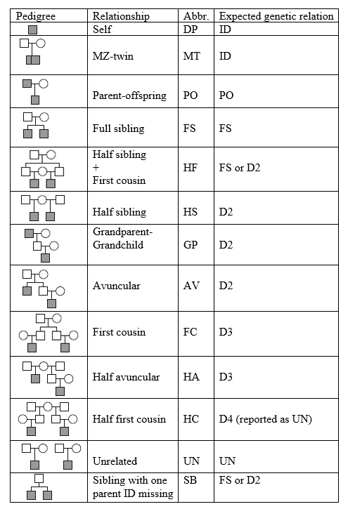
Ped relation: relationship derived from subject sample mapping file and pedigree file (See Table 1 for code meanings).
p_value: probability that the genetic relationship is NOT the predicted type
Table 1. Pedigree relationships and the expected genetic relationships
.
When multiple PLINK sets are checked pairwise, the output file will have two extra columns, DS1 and DS2, showing the dataset IDs for the pair of PLINK sets.
PlotGraf.pl to plot closely related subjectsPlotGraf.pl is a perl script that plots graphs to show the distributions of HGMR and AGMR values of the related pairs of subjects. It shows brief instructions when it is executed without parameters:
$ PlotGraf.pl

Usage: PlotGraf.pl <input related subject file> <output png file> <graph type> [Options]

Note:
    Valid graph types are:
        1 = HGMR histogram
        2 = AGMR histogram
        3 = HGMR + AGMR scatter plot

Options:
    -gw     graph width:  Set graph width in pixels
    -gh     graph height: Set graph height in pixels
    -xmax   max x value:  Set maximum HGMR or AGMR on x-axis of the histogram
    -ymax   max y value:  Set maximum number of pairs on y-axis of the histogram
    -dot    size:         Set dot size in pixels on the scatter plot
    -hfd    size:         Set dot size in pixels for HF (half sibling + full cousin) pairs
It takes three required parameters. The first parameter should be the name of the file that is generated by graf and contains related subject pairs. The second is the output .png file which shows the graph. The third is an integer representing the graph type. The options should be entered after the required parameters. Below are some examples showing how to run the script.
$ graf -plink data/affy_hapmap -maxhm 15 -ssm data/affy_hapmap_ssm.txt -ped data/affy_hapmap_fake_pedigree.txt -out data/affy_hapmap_rels_15.txt
$ PlotGraf.pl data/affy_hapmap_rels_15.txt data/affy_hapmap_hgmr.png 1
$ PlotGraf.pl data/affy_hapmap_rels_15.txt data/affy_hapmap_agmr.png 2
$ PlotGraf.pl data/affy_hapmap_rels_15.txt data/affy_hapmap_scatter.png 3
In the first step the C++ program finds related pairs and saves the results to affy_hapmap_rels_15.txt. Then PlotGraf.pl takes the results and plots histograms to show distributions of HGMR values of the related subjects, AGMR values of the duplicates, and a scatter plot to show distribution of both values.
In both histograms, the colored bars represent different types of relationships derived from the SSM and pedigree files (see Table 1 for the meanings of the two-letter abbreviations). The cyan lines show the cutoff values suggested by GRAF to separate different types of relationships determined by comparing the genotypes. In the scatter plot, each contour line shows the area that is predicted to contain 95% of the pairs for each relatedness type, assuming that all 10,000 fingerprinting SNPs are genotyped for all of the subjects in a large, homogeneous, random mating population. Note that the HapMap samples were collected from human individuals from very different populations, and GRAF is more accurate when predicting relatedness for subjects from a homogeneous population.
$ graf -plink data/affy_hapmap -maxhm 15 -ssm data/affy_hapmap_fake_ssm.txt -ped data/affy_hapmap_fake_pedigree.txt -out data/affy_hapmap_fake_rels.txt
$ PlotGraf.pl data/affy_hapmap_fake_rels.txt data/affy_hapmap_hgmr_f1.png 1 -gw 1000 -gh 500
$ PlotGraf.pl data/affy_hapmap_fake_rels.txt data/affy_hapmap_agmr_f1.png 2 -xmax 60 -ymax 20
$ PlotGraf.pl data/affy_hapmap_fake_rels.txt data/affy_hapmap_scatter_f1.png 3 -dot 5
The above examples show that graph size, axis limits and the scatter plot dot size can be adjusted by users. In the first step a fake pedigree and a fake SSM file are used to show how GRAF finds and reports errors in the pedigree and SSM files. The HGMR histogram generated in the second step shows that some of the related pairs reported by the pedigree and SSM file don’t match the genetic relatedness determined by GRAF. It also shows that the graph size can be adjusted by using options -gw and -gh. The AGMR histogram also shows the mismatches between the relationship types reported in the input files and those determined by GRAF. The axis limits can be adjusted by using -xmax and -ymax options. The scatter plot shows that the dot size can be adjusted using -dot option.
Multiple genotype datasets can be combined into one .fpg file and passed to graf for determining genetic relationships, e.g.,
$ graf -exfp data/affy_hapmap,data/perlegen_hapmap -out data/comb_hapmap.fpg
$ graf -geno data/comb_hapmap.fpg -out data/comb_hapmap_rels.txt -maxhm 15 -ped data/affy_hapmap_fake_pedigree.txt -ssm data/comb_hapmap_ssm.txt
$ PlotGraf.pl data/comb_hapmap_rels.txt data/comb_hapmap_hgmr.png 1
$ PlotGraf.pl data/comb_hapmap_rels.txt data/comb_hapmap_agmr.png 2
$ PlotGraf.pl data/comb_hapmap_rels.txt data/comb_hapmap_scatter.png 3
When multiple datasets are used, if there are no SSM and pedigree files, it is not required that the sample and subject IDs be unique across datasets. GRAF uses both DS# and subject/sample IDs to identify subjects or samples. In the output table, GRAF shows both the DS# and ID for each subject or sample. However, when there are SSM and pedigree files, it is required that IDs be unique across datasets. GRAF doesn’t take multiple SSM or pedigree files. The user needs to combine multiple SSM or pedigree files into one, and each ID in the combined SSM or pedigree file should represent only one sample or subject. Neither the SSM file nor the pedigree file has DS# columns.
The -hfd option of PlotGraf.pl lets the user set the dot size for the half sibling + full cousin pairs (HF, see Table 1) in the scatter plot. The HF relationship is genetically remoter than full sibling but closer than second degree relatives. In the scatter plot, these pairs are predicted to be between FS and D2 pairs. In the rare cases when there are HF pairs, the user can use -hfd option to highlight the HF pairs by setting different dot sizes for them.
GRAF-pop calculates genetic distances from each subject to several reference populations and estimates subject ancestry and ancestral proportions based on these distances (Jin et al., 2019). Four genetic distances scores, GD1, GD2, GD3, GD4, are used in ancestry inference in the current version of GRAF. Subjects in the input datasets are clustered using these scores and plotted on scatter plots.
GRAF-pop assumes that each subject is an admixture of three ancestries: European (E), African (F), and Asian (A), and estimates ancestral proportions Pe, Pf, Pa based on GD1 and GD2 scores using barycentric coordinates. It also assigns a population ID (PopID) to each subject using the cutoff values shown in Tables 2 and 3.
Table 2. Grouping subjects based on the ancestry proportions
| PopID | Population | Cutoff standard |
|---|---|---|
| 1 | European | Pe ≥ 87% |
| 2 | African | Pf ≥ 95% |
| 3 | East Asian | Pa ≥ 95% |
| 4 | African American | 40% ≤ Pf < 95% and Pa < 13% |
| 5 | Latin American 1 | Pf < 40% and Pe < 87% and Pa < 13% and Pf ≥ Pa |
| 6,7,8 | (Three populations) | Pa < 95% and Pe < 87% and Pf < 13% and Pf < Pa |
| 9 | Other | Pa ≥ 13% and Pf ≥ 13% |
Table 3. Separating Asians and Latin Americans using GD1 and GD4 scores
| PopID | Population | Cutoff standard |
|---|---|---|
| 7 | Asian-Pacific Islander | GD1 > 30 × (GD4)2 + 1.73 |
| 8 | South Asian | GD4 > 5 × (GD1 -1.69)2 + 0.042 |
| 6 | Latin American 2 | GD4 < 0 and PopID is not 7 |
As in GRAF-rel, GRAF-pop takes genotype datasets in either PLINK format (.fam, .bim, .bed) or GRAF format (.fpg). In addition, GRAF-pop can read self-reported ancestries from the input file and compare the ancestries inferred from genotypes with the self-reported ones. The input file should be a plain text file with two columns (without column header), containing subject ID and the self-reported ancestry, respectively.
graf to infer subject ancestryOption -pop is used by graf to infer subject ancestry:
$ graf

Usage: graf [options]
    -pop    output file:     Check subject populations and save results to the output file
The following command determines population structures and saves results to the output file:
graf -plink data/G1000FpGeno -pop data/G1000_sbj_scores.txt
PlotPopulations.pl to plot population resultsThe results generated by graf can be passed to PlotPopulations.pl for further processing. The following instructions are displayed on the screen when the script is run without parameters:
$ PlotPopulations.pl

Usage: PlotPopulations.pl <input file> <output file> [Options]

Note:
    Output file should be either a .png file or a .txt file.

    If the output file is a .png file, the script will plot the results to a graph and save the graph to the file.
    If the output file is a .txt file, the script will save the calculated subject ancestry components to the file.

Options:
    Set window size in pixels
        -gw      graph width

    Set graph axis limits
        -xmin    min x value
        -xmax    max x value
        -ymin    min y value
        -ymax    max y value

    Set a rectangle area to retrieve subjects for graph of GD1 vs. GD2
        -xcmin   min x value
        -xcmax   max x value
        -ycmin   min y value
        -ycmax   max y value
        -isByd   0 or 1
                 0:  retrieve subjects whose values are within the above rectangle (default value)
                 1:  retrieve subjects whose values are beyond the above rectangle

    Set population cutoff lines
        -ecut   proportion: cutoff European proportion dividing Europeans from other population. Default 87%.
        -fcut   proportion: cutoff African proportion dividing Africans from other population. Default 95%.
                            Set it to -1 to combine African and African American populations
        -acut   proportion: cutoff East Asian proportion dividing East Asians from other populations. Default 95%.
                            Set it to -1 to combine East Asian and Asian-Pacific Islander populations
        -ohcut  proportion: cutoff African proportion dividing Latin Americans from Other population. Default 13%.
        -fhcut  proportion: cutoff African proportion dividing Latin Americans from African Americans. Default 40%.

    Select some self-reported populations (by IDs) to be highlighted on the graph
        -pops   comma-separated population IDs, e.g., -pops 1,3,4 -> highlight populations #1, #3, and #4

    Select self-reported populations (by IDs) to show areas including 95% dbGaP subjects with genotypes of at least 4000 fingerprint SNPs
        -areas  comma-separated dbGaP self-population IDs, e.g., -areas 1,3
            -> show areas that include 95% dbGaP subjects with self-reported populations #1 and #3
              1: European
              2: African
              3: East Asian
              4: African American
              5: Latin American 1
              6: Latin American 2
              7: Asian-Pacific Islander
              8: South Asian

    Select which score to show on the y-axis
        -gd4     1 or 0.  1: show GD4 on y-axis;  0: show GD2

    Set population cutoff lines
        -cutoff  1 or 0.  1: show cutoff lines;  0: hide cutoff lines

    Rotate the plot with respect to the x-axis by a certain angle
        -rotx    angle in degrees

    Set the size (diameter) of each dot that represents each subject
        -dot     pixels

    The input file with self-reported subject race information
        -spf     a file with two columns: subject and self-reported population
The script takes two required parameters, which must be the first two arguments and are not preceded by flags, unlike all the optional arguments, which are preceded by a flag. The first parameter should be the name of the file that is generated by graf -pop option and contains subject genetic distance scores. The second parameter is the output file, expected to be either a .png or .txt file. If the output file is a .png file, the script processes the scores and saves the results to the output file. The default graph is GD1 vs. GD2, e.g.,
$ graf -plink data/G1000FpGeno -pop data/G1000_sbj_scores.txt
$ PlotPopulations.pl data/G1000_sbj_scores.txt data/G1000_sbj_pops.png
When option -gd4 is set to 1, the script generates a graph of GD1 vs. GD4:
$ PlotPopulations.pl data/G1000_sbj_scores.txt data/G1000_sbj_pops_gd4.png -gd4 1
If the output file is a .txt file, the script processes the data and saves the results to the output file in a format of a rectangular table.
$ PlotPopulations.pl data/G1000_sbj_scores.txt data/G1000_sbj_list.txt
In the output file, columns P_e, P_f, P_a show each subject’s African, European, and East Asian proportions Pe, Pf, Pa, in percentages. The populations determined by GRAF-pop are included in the last two columns as an identifier and as the full name of the population.
When self-reported ancestries are available, the information can be passed to the script with -spf option so that the script can color-code the subjects using the self-reported ancestries, e.g.,
$ PlotPopulations.pl data/G1000_sbj_scores.txt data/G1000_sbj_pops_sp.png -spf data/G1000SbjSuperPop.txt
The format of the input ancestry file is described above. In the graph generated by the script, the ancestries are numbered and color coded.
The cutoff lines used to partition the subjects are drawn on the graphs when option -cutoff is set, e.g.,
$ PlotPopulations.pl data/G1000_sbj_scores.txt data/G1000_sbj_pops_cut.png -spf data/G1000SbjSuperPop.txt -cutoff 1
$ PlotPopulations.pl data/G1000_sbj_scores.txt data/G1000_sbj_pops_cut_gd4.png -spf data/G1000SbjSuperPop.txt -gd4 1 -cutoff 1
If multiple subjects appear at the same locations in the x-y plane, the user can use option -pops to bring some ancestries to the front, while setting some ancestries to the back and fade them out in the graph. For example, the following command generates a graph with the ancestry No. 5 (AMR, standing for Ad Mixed American) in the back and colored yellow. The assignments of colors to populations are currently hard-coded.
$ PlotPopulations.pl data/G1000_sbj_scores.txt data/G1000_sbj_pops_1234.png -spf data/G1000SbjSuperPop.txt -pops 1,3,2,4
The ancestry numbers following -pops should be separated by commas without spaces.
One can also use the -rotx option to rotate the graph of GD2 vs. GD1 around x-axis by a certain angle specified in degrees (can be any real number). For example, the following command generates a graph showing the subjects rotated by 90°:
$ PlotPopulations.pl data/G1000_sbj_scores.txt data/G1000_sbj_pops_90.png -spf data/G1000SbjSuperPop.txt -rotx 90
Options -gw, -xmin, -xmax, -ymin, -ymax, -dot, similar to those in PlotGraf.pl, can be used to adjust the graph size, specify axis limits, and set the dot size, e.g.,
$ PlotPopulations.pl data/G1000_sbj_scores.txt data/G1000_sbj_pops_gw.png -spf data/G1000SbjSuperPop.txt -gw 800 -ymin 1.1 -dot 5
$ PlotPopulations.pl data/G1000_sbj_scores.txt data/G1000_sbj_pops_gw_gd4.png -spf data/G1000SbjSuperPop.txt -gw 800 -gd4 1 -ymin -0.2
One can use the option -areas to select populations to show the expected oval areas that include 95% of dbGaP subjects with at least 4000 fingerprint SNPs with genotypes, e.g.,
$ PlotPopulations.pl data/G1000_sbj_scores.txt data/G1000_sbj_pops_a.png -spf data/G1000SbjSuperPop.txt -areas 1,4,7
The integers in the comma-delimited string represent the eight self-reported ancestry groups in dbGaP, with most common ancestry terms in each group shown below:
            1: European
            2: African
            3: East Asian
            4: African American
            5: Latin American 1
            6: Latin American 2
            7: Asian-Pacific Islander
            8: South Asian
GRAF-pop uses the ancestry proportions shown in Tables 2 and 3 as default cutoff values. The user can use options -ecut, -fcut, -acut, -ohcut, -ahcut, -fhcut to set the cutoff values to different numbers, e.g.,
$ PlotPopulations.pl data/G1000_sbj_scores.txt data/G1000_sbj_pops_ucut.png -spf data/G1000SbjSuperPop.txt -cutoff 1 -fcut 85 -ahcut 80 -ohcut 15.5
When -fcut or -acut are set to negative values, the African or East Asian cutoff line is not plotted on the graph, and the script does not distinguish Africans from African Americans, or East Asians from Asian-Pacific Islanders, e.g.,
$ PlotPopulations.pl data/G1000_sbj_scores.txt data/G1000_sbj_pops_nf.png -spf data/G1000SbjSuperPop.txt -cutoff 1 -fcut -1
As mentioned above, when the second parameter (the output file) is a .txt file, the script saves subjects and ancestry proportions into a rectangular table. Options -xcmin, -xcmax, -ycmin, -ycmax, -isByd can be used to specify a rectangular area and let the script retrieve subjects whose x(GD1), y(GD2) scores are either within or beyond this area. For example, the following command saves all subjects with 1.8 < GD1 < ∞ and -∞ < GD2 < 1.2, which are all the EAS (East Asian) subjects:
$ PlotPopulations.pl data/G1000_sbj_scores.txt data/G1000_sbj_list_cut.txt -spf data/G1000SbjSuperPop.txt -xcmin 1.8 -ycmax 1.2
When option -isByd is set to 1, the script retrieves subjects whose values are beyond the rectangular area specified by options -xcmin, -xcmax, -ycmin, -ycmax. For example, the following command excludes most of the 1000 Genomes Project’s subjects with super populations AMR (Ad Mixed American) and SAS (South Asian):
$ PlotPopulations.pl data/G1000_sbj_scores.txt data/G1000_sbj_list_cutb.txt -spf data/G1000SbjSuperPop.txt -xcmin 1.64 -xcmax 1.8 -ycmin 1.24 -ycmax 1.36 -isByd 1
GRAF-sex calculates heterozygosity rate of genotypes of pre-selected 1000 SNPs on X-chromosome and determines the genotype sex and compares it with the self-reported phenotype sex for each subject.
As in GRAF-rel and GRAF-pop, GRAF-sex takes genotype datasets in either PLINK format (.fam, .bim, .bed) or GRAF format (.fpg). In addition, GRAF-rel can read self-reported sexes either from the PLINK .fam file or a separate input file and compares the sexes determined using genotypes with the self-reported phenotyep sexes. The input file should be a plain text file with two columns, containing sample ID and the self-reported phenotype sexes, respectively.
graf to determine genotype sexOption -sex is used by graf to determine genotype sex:
$ graf

Usage: graf [options]
    -sex    output file:     Do sex check using fingerprint genotypes on X-chromosome and save results to the output file
The following command determines sample genotype sexes and saves results to the output file:
$ graf -plink data/SexTestDs01 -sex data/SexTestRes01.txt
PlotSexCheckResults.pl to plot sex check resultsThe results generated by graf can be passed to PlotSexCheckResults.pl for plotting. The following instructions are displayed on the screen when the script is run without parameters:
$ PlotSexCheckResults.pl

Usage: PlotSexCheckResults.pl [Options]

Options:
    Specify input and output files
        -in      (required) input file generated by graf with -sex option
        -out     (required) output .png file to save the graph plotted by the script
        -sum     output .txt file to save the summary generated by the script
        -sf      two-column plain text file including sample sexes (1=male; 2=female)

    Set window size in pixels and axis scale
        -gw      graph width
        -gh      graph height
        -ymax    max number of samples to plot on y-axis

    Set cutoff heterozygosity rates (%)
        -mhr     maximum heterozygosity rate of male samples
        -fhr1    minimum heterozygosity rate of female samples
        -fhr2    maximum heterozygosity rate of female samples
The script takes two required parameters, the input and output files, passed in though -in and -out options.
$ graf -plink data/SexTestDs01 -sex data/SexTestRes01.txt
$ PlotSexCheckResults.pl -in data/SexTestRes01.txt -out data/SexTestRes01.png
The script plots the results in input file data/SexTestRes01.txt and saves the graph to data/SexTestRes01.png.
By default, PlotSexCheckResults.pl reads self-reported phenotype sexes from the .fam file of the PLINK set. The user can specify another file for the script to read the phenotype sexes, e.g.,
$ PlotSexCheckResults.pl -in data/SexTestRes01.txt -out data/SexTestRes01b.png -sf data/SexTestSmpSex02.txt
The user can use option -sum to save the summary into a specified file, e.g.,
$ PlotSexCheckResults.pl -in data/SexTestRes01.txt -out data/SexTestRes01b.png -sf data/SexTestSmpSex02.txt -sum data/SexTestRes01_sum.txt
Option -ymax can be used to adjust the y-axis scale, e.g.,
$ PlotSexCheckResults.pl -in data/SexTestRes01.txt -out data/SexTestRes01c.png -sf data/SexTestSmpSex02.txt -sum data/SexTestRes01_sum.txt -ymax 30
Graph size can be adjusted using options -gw and -gh, e.g.,
$ PlotSexCheckResults.pl -in data/SexTestRes01.txt -out data/SexTestRes01d.png -sf data/SexTestSmpSex02.txt -ymax 25 -gw 800 -gh 400
The user can set cutoff heterozygosity rates (in percentage) using options -mhr (maximum heterozygosity rate of male samples), -fhr1 (minimum heterozygosity rate of female samples) and -fhr2 (maximum heterozygosity rate of female samples), e.g.,
$ PlotSexCheckResults.pl -in data/SexTestRes01.txt -out data/SexTestRes01e.png -sf data/SexTestSmpSex02.txt -ymax 25 -fhr1 34 -fhr2 52 -sum data/SexTestRes01e_sum.txt
SetRsIdsInBimFile.pl to convert SNP IDs in .bim file into RS IDsgraf requires that SNP IDs in the .bim be RS IDs. If they are not RS IDs, the user can use SetRsIdsInBimFile.pl to convert them into RS IDs.
$ SetRsIdsInBimFile.pl

This script checks chromosome and position for each SNPs in the PLINK .bim file to determine
if it is a GRAF fingerprint SNPs. Assuming genome build GRCh 37 or 38, the script does the following:

    if the SNP is a GRAF fingerprint SNP then
        if the SNP ID is an RS ID then
            if the SNP ID is different from that expected based on chromosome and position then
                replace the SNP ID as "RS_ID_conflict"
                report it in the WARNING message
        else
            replace the SNP ID with rs ID

If output file is specified, it saves the new results to the output file. Otherwise it updates the input file and saves the original .bim file to <plink_set_basename>_orig.bim

Usage: SetRsIdsInBimFile.pl <plink_bim_file> [output_bim_file]
For example, no sex check results are generated after the following command is run, since graf doesn’t find any fingerprint SNPs on X-chromosome:
$ graf -plink data/SexTestDs02 -sex data/SexTestRes02.txt
We can do sex check in the following two steps:
$ SetRsIdsInBimFile.pl data/SexTestDs02.bim
$ graf -plink data/SexTestDs02 -sex data/SexTestRes02.txt
SetRsIdsInBimFile.pl converts fingerprint SNPs to RS IDs on all chromosomes, which means it can be used for relationship, population and sex checks.
Jin Y, Schäffer AA, Sherry ST, and Feolo M (2017). Quickly identifying identical and closely related subjects in large databases using genotype data. PLoS One. 12(6):e0179106.
Jin Y, Schäffer AA, Feolo M, Holmes JB and Kattman BL (2019). GRAF-pop: A Fast Distance-based Method to Infer Subject Ancestry from Multiple Genotype Datasets without Principal Components Analysis. G3: Genes | Genomes | Genetics. August 1, 2019 vol. 9 no. 8 2447-2461.